Differential analysis
This notebook shows how to create a differential analysis based on two CombObj’s (A and B) from two different cell types.
[1]:
import tfcomb.objects
Prepare GM12878 and K562 CombObjs
The two objects contain ENCODE ChIP-seq peaks (1bp centered on the middle of the peak) from the celltypes GM12878 and K562 respectively.
[2]:
A = tfcomb.objects.CombObj(verbosity=0)
A.prefix = "GM12878"
A.TFBS_from_bed("../data/GM12878_hg38_chr4_TF_chipseq.bed")
A.market_basket()
A.set_verbosity(1) #reset verbosity to INFO
Internal counts for 'TF_counts' were not set. Please run .count_within() to obtain TF-TF co-occurrence counts.
[3]:
B = tfcomb.objects.CombObj(verbosity=0)
B.prefix = "K562"
B.TFBS_from_bed("../data/K562_hg38_chr4_TF_chipseq.bed")
B.market_basket()
Internal counts for 'TF_counts' were not set. Please run .count_within() to obtain TF-TF co-occurrence counts.
Compare two CombObj’s
The two objects contain different amounts of TFs and rules:
[4]:
print(A)
print(B)
<CombObj: 112109 TFBS (151 unique names) | Market basket analysis: 21284 rules>
<CombObj: 216370 TFBS (447 unique names) | Market basket analysis: 166088 rules>
We will now use the .compare-function of CombObj ‘A’ to directly compare it with CombObj ‘B’. What you will see is that many of the TFs are different between the object and are thus removed:
[5]:
compare_obj = A.compare(B)
WARNING: 365 TFs were not common between objects and were excluded from .rules. Set 'join' to 'outer' in order to use all TFs across objects. The TFs excluded were: ['TEAD2', 'ZNF215', 'NR3C1', 'MEF2C', 'ZNF263', 'AGO1', 'ZEB1', 'ZEB2', 'ILF3', 'ZNF584', 'POLR3A', 'XRCC3', 'KDM5B', 'POLR2G', 'PBX3', 'KLF5', 'ZNF695', 'NFRKB', 'SAP30', 'GTF2A2', 'CC2D1A', 'MAFG', 'ZNF197', 'RBM22', 'MCM3', 'IRF9', 'XRCC5', 'MCM7', 'THAP12', 'HNRNPK', 'TRIP13', 'ZNF764', 'TFE3', 'U2AF1', 'JUN', 'ETV5', 'SNAPC5', 'KLF1', 'ZNF830', 'ZNF444', 'ZFP91', 'ZNF354B', 'GTF2F1', 'LEF1', 'ZBTB8A', 'MYB', 'ZC3H8', 'NCOA4', 'KLF6', 'POLR2H', 'STAT3', 'BCOR', 'ZNF165', 'POU2F2', 'ZNF644', 'DACH1', 'SMARCB1', 'IKZF2', 'HEY1', 'PTTG1', 'BATF', 'MEF2D', 'FIP1L1', 'FOXJ2', 'YBX3', 'BRD9', 'ZNF217', 'RBM34', 'DLX4', 'ZNF75A', 'ZSCAN32', 'PBX2', 'ZNF84', 'PHB', 'SP2', 'PHF20', 'POU5F1', 'CCAR2', 'FOXA1', 'PATZ1', 'ZNF274', 'ZNF148', 'MNT', 'HLTF', 'HDAC3', 'ZNF175', 'ZNF436', 'ATF1', 'ZNF311', 'ELF4', 'HDAC1', 'ZNF507', 'ZFP1', 'RBM15', 'PRDM15', 'ZBTB7A', 'ARID2', 'TAL1', 'ZNF3', 'ERF', 'TFCP2', 'NR2F2', 'ZFX', 'ELF2', 'PAX8', 'STAG1', 'ZNF184', 'NCOR1', 'ZNF551', 'SIN3B', 'ZBTB2', 'TBX21', 'KHSRP', 'PTBP1', 'THAP7', 'NELFE', 'RBFOX2', 'ARID3B', 'PHF21A', 'EP400', 'ZNF700', 'WRNIP1', 'MYNN', 'FOSL1', 'HNRNPLL', 'SMARCE1', 'TEAD1', 'ZBTB11', 'ZNF655', 'RELA', 'HNRNPL', 'SMARCA4', 'HMBOX1', 'PRMT5', 'ZNF83', 'PCBP2', 'E2F1', 'SUPT5H', 'HIVEP1', 'ZNF257', 'TOE1', 'ZKSCAN1', 'ZNF76', 'RBPJ', 'CGGBP1', 'PAX5', 'ZNF282', 'U2AF2', 'CBX2', 'ID3', 'NEUROD1', 'PCBP1', 'ZNF445', 'CBX1', 'FOXO4', 'MAFF', 'ARID1B', 'CHAMP1', 'PHF8', 'ETV1', 'SOX6', 'ZNF407', 'GTF2E2', 'ZNF589', 'ATF6', 'TRIM24', 'TBX18', 'ADNP', 'KLF10', 'E2F6', 'BCL3', 'ZNF174', 'ZNF57', 'ZNF639', 'ZNF319', 'NR2F6', 'GABPB1', 'SNIP1', 'MGA', 'SRSF7', 'RUNX1', 'E2F3', 'SIRT6', 'CBFA2T2', 'TRIM28', 'HDAC8', 'ELK3', 'ASH2L', 'KDM4B', 'ZNF622', 'CREB3L1', 'ZNF79', 'EHMT2', 'C11orf30', 'HSF1', 'ZBTB17', 'ZMYM3', 'ZNF281', 'CLOCK', 'BDP1', 'ZNF395', 'ZNF250', 'TSHZ1', 'TFDP1', 'BCL11A', 'STAT1', 'CTBP1', 'HES1', 'TBPL1', 'IRF4', 'DIDO1', 'SFPQ', 'PYGO2', 'ZNF133', 'GATAD2A', 'ZNF280B', 'RBM39', 'EBF1', 'POLR2B', 'HNRNPUL1', 'ZNF397', 'CDC5L', 'ZC3H11A', 'IRF3', 'BCL6', 'ZBTB12', 'KLF13', 'MCM5', 'SMARCC2', 'ZNF408', 'NR0B1', 'ZNF518B', 'ZKSCAN8', 'NR1H2', 'ZC3H4', 'ZNF780A', 'ZNF146', 'CHD7', 'ZNF717', 'RUNX3', 'E2F7', 'ZKSCAN3', 'WHSC1', 'HOMEZ', 'TRIM25', 'CREB5', 'FOXJ3', 'ZNF280A', 'DEAF1', 'IRF1', 'HMG20B', 'MBD2', 'PHTF2', 'GMEB1', 'TCF7L2', 'MCM2', 'NFATC1', 'BRD4', 'ILK', 'TAF15', 'MTA1', 'SNRNP70', 'RNF2', 'RLF', 'ZBTB9', 'NFIX', 'ZBTB5', 'IRF2', 'ESRRB', 'COPS2', 'ARHGAP35', 'ZNF687', 'ZNF23', 'DDX20', 'MEIS2', 'MEF2B', 'ASH1L', 'SRSF1', 'FUS', 'NFE2', 'HMGN3', 'EWSR1', 'KAT2B', 'SRSF3', 'ZNF239', 'TRIM22', 'RBM17', 'CSDE1', 'RREB1', 'MIER1', 'GATA2', 'NFE2L1', 'CREBBP', 'HNRNPH1', 'ZNF7', 'RFX1', 'STAT5B', 'TAF7', 'KAT8', 'KLF16', 'ZNF778', 'TAF9B', 'PTRF', 'MYBL2', 'ZNF12', 'ZNF316', 'ZNF207', 'PHB2', 'ATF4', 'TEAD4', 'ZNF212', 'NUFIP1', 'RXRA', 'GATA1', 'ETS2', 'GTF2I', 'NCOA2', 'SAFB', 'NR4A1', 'PRPF4', 'MITF', 'THAP1', 'L3MBTL2', 'ZNF740', 'VEZF1', 'ZNF583', 'RBM25', 'TSC22D4', 'DNMT1', 'GTF3C2', 'THRA', 'IRF5', 'HINFP', 'ZMIZ1', 'ZNF785', 'GTF2B', 'CREB3', 'NONO', 'ZNF77', 'CBX8', 'ZNF318', 'RBM14', 'PRDM10', 'SETDB1', 'ZNF512', 'KAT2A', 'NCOA1', 'ZNF766', 'EED', 'SHOX2', 'ZHX1', 'CCNT2', 'RELB', 'CBFA2T3', 'AFF1', 'E2F5', 'SAFB2', 'CEBPG', 'DDIT3', 'CTCFL', 'THRAP3', 'NCOA6', 'RFX7', 'ZNF324', 'ZNF347']
INFO: Calculating foldchange for contrast: GM12878 / K562
INFO: The calculated log2fc's are found in the rules table (<DiffCombObj>.rules)
The results of the differential analysis are now found in the .rules of the CombObj:
[6]:
compare_obj.rules
[6]:
| TF1 | TF2 | GM12878_cosine | K562_cosine | GM12878/K562_cosine_log2fc | |
|---|---|---|---|---|---|
| SIX5-SUZ12 | SIX5 | SUZ12 | 0.005640 | 0.478929 | -4.966291 |
| SUZ12-SIX5 | SUZ12 | SIX5 | 0.005640 | 0.478929 | -4.966291 |
| SUZ12-HCFC1 | SUZ12 | HCFC1 | 0.004308 | 0.282011 | -4.351172 |
| HCFC1-SUZ12 | HCFC1 | SUZ12 | 0.004308 | 0.282011 | -4.351172 |
| UBTF-SKIL | UBTF | SKIL | 0.004266 | 0.253694 | -4.208163 |
| ... | ... | ... | ... | ... | ... |
| POLR2AphosphoS2-MAX | POLR2AphosphoS2 | MAX | 0.206904 | 0.002029 | 4.172457 |
| ELF1-POLR2AphosphoS2 | ELF1 | POLR2AphosphoS2 | 0.245057 | 0.003654 | 4.223385 |
| POLR2AphosphoS2-ELF1 | POLR2AphosphoS2 | ELF1 | 0.245057 | 0.003654 | 4.223385 |
| POLR2AphosphoS2-TBP | POLR2AphosphoS2 | TBP | 0.254481 | 0.003560 | 4.285724 |
| TBP-POLR2AphosphoS2 | TBP | POLR2AphosphoS2 | 0.254481 | 0.003560 | 4.285724 |
12114 rows × 5 columns
Plot differential co-occurring TFs
We can now have a look at the changes between the two objects in terms of ‘cosine’ measure:
[7]:
compare_obj.plot_heatmap()

Like in the case for CombObjs, we can also select a subset of interesting differentially co-occurring TFs:
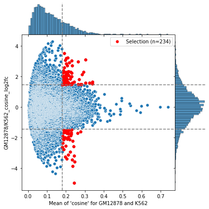
[8]:
selection = compare_obj.select_rules(measure_threshold_percent=0.2)
INFO: Selecting rules for contrast: ('GM12878', 'K562')
INFO: measure_threshold is None; trying to calculate optimal threshold
INFO: mean_threshold is None; trying to calculate optimal threshold
INFO: Creating subset of rules using thresholds

We can also plot the network to show the pairs which are either increasing or decreasing in ‘cosine’ measure between the two cell types:
[9]:
selection.plot_network()
INFO: Finished! The network is found within <CombObj>.network.
[9]:

The strictness of the automatic threshold can be adjusted with measure_threshold_percent and mean_threshold_percent:
[10]:
selection2 = compare_obj.select_rules(measure_threshold_percent=0.1, mean_threshold_percent=0.2)
INFO: Selecting rules for contrast: ('GM12878', 'K562')
INFO: measure_threshold is None; trying to calculate optimal threshold
INFO: mean_threshold is None; trying to calculate optimal threshold
INFO: Creating subset of rules using thresholds
[11]:
selection2.plot_network()
INFO: Finished! The network is found within <CombObj>.network.
[11]:

It is also possible to set specific thresholds with measure_threshold and mean_threshold (these will overwrite the automatic thresholding set by measure_threshold_percent and mean_threshold_percent):
[12]:
selection3 = compare_obj.select_rules(measure_threshold=(-2,2), mean_threshold=0)
INFO: Selecting rules for contrast: ('GM12878', 'K562')
INFO: Creating subset of rules using thresholds

[13]:
selection3.plot_network()
INFO: Finished! The network is found within <CombObj>.network.
[13]:
