Orientation analysis

This is an example of a orientation analysis using .TFBS from motif sites.

Create CombObj and fill it with .TFBS from motif scanning

[1]:

import tfcomb
C = tfcomb.CombObj(verbosity=0)

[2]:

C.TFBS_from_motifs(regions="../data/GM12878_hg38_chr4_ATAC_peaks.bed",
                   motifs="../data/HOCOMOCOv11_HUMAN_motifs.txt",
                   genome="../data/hg38_chr4_masked.fa.gz",
                   threads=8)

For this analysis, we will run count_within() with the stranded option turned on:

[3]:

C.count_within(stranded=True, threads=8)
C.market_basket()

[4]:

C.rules

[4]:

	TF1	TF2	TF1_TF2_count	TF1_count	TF2_count	cosine	zscore
KLF1(-)-KLF9(-)	KLF1(-)	KLF9(-)	145	291	209	0.587961	66.330168
KLF9(-)-KLF1(-)	KLF9(-)	KLF1(-)	145	209	291	0.587961	66.330168
KLF1(-)-KLF12(-)	KLF1(-)	KLF12(-)	152	291	240	0.575164	61.565308
KLF12(-)-KLF1(-)	KLF12(-)	KLF1(-)	152	240	291	0.575164	61.565308
KLF12(-)-KLF9(-)	KLF12(-)	KLF9(-)	127	240	209	0.567055	62.215597
...	...	...	...	...	...	...	...
STAT2(+)-SP1(+)	STAT2(+)	SP1(+)	1	556	636	0.001682	-5.135968
NFE2L1(+)-SP2(+)	NFE2L1(+)	SP2(+)	1	451	798	0.001667	-4.294191
SP2(+)-NFE2L1(+)	SP2(+)	NFE2L1(+)	1	798	451	0.001667	-4.294191
BCL11A(+)-SP1(-)	BCL11A(+)	SP1(-)	1	562	653	0.001651	-4.399691
SP1(-)-BCL11A(+)	SP1(-)	BCL11A(+)	1	653	562	0.001651	-4.399691

226676 rows × 7 columns

Analyze preferential orientation of motifs

First, we create a directionality analysis for the rules found:

[5]:

df = C.analyze_orientation()

INFO: Rules are symmetric - scenarios counted are: ['same', 'opposite']

[6]:

df.head()

[6]:

	TF1	TF2	TF1_TF2_count	same	opposite	std	pvalue
SP3-SP4	SP3	SP4	534	0.758427	0.241573	0.365471	7.004689e-33
PATZ1-SP1	PATZ1	SP1	631	0.730586	0.269414	0.326098	4.936837e-31
PATZ1-SP3	PATZ1	SP3	642	0.725857	0.274143	0.319410	2.479952e-30
SP1-SP3	SP1	SP3	756	0.705026	0.294974	0.289951	1.751909e-29
KLF1-KLF9	KLF1	KLF9	243	0.851852	0.148148	0.497594	5.347598e-28

We can subset these on pvalue and number of sites:

[7]:

selected = df[(df["pvalue"] < 0.01) & (df["TF1_TF2_count"] > 50)]

[8]:

#Number of TF pairs with significant differences in orientation
selected.shape[0]

[8]:

We can also use the .loc-operator of the pandas dataframe to show the results of a subset of TF1-TF2-pairs:

[9]:

df.loc[["EGR1-IRF4", "SP1-TAF1"]]

[9]:

	TF1	TF2	TF1_TF2_count	same	opposite	std	pvalue
EGR1-IRF4	EGR1	IRF4	15	0.866667	0.133333	0.518545	0.004509
SP1-TAF1	SP1	TAF1	153	0.679739	0.320261	0.254189	0.000009

Visualization of orientation preference

[10]:

_ = selected.plot_heatmap()

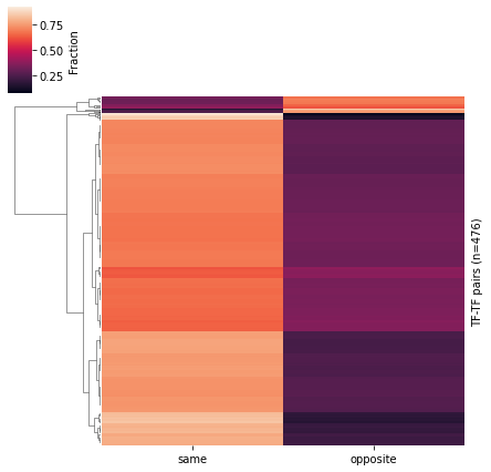
../_images/examples_Orientation_analysis_18_0.png

We can select the subsets by investigating the selected pairs:

[11]:

selected.sort_values("same").head(5)

[11]:

	TF1	TF2	TF1_TF2_count	same	opposite	std	pvalue
KLF3-ZIC3	KLF3	ZIC3	66	0.166667	0.833333	0.471405	6.093838e-08
SP1-ZFX	SP1	ZFX	81	0.222222	0.777778	0.392837	5.733031e-07
PATZ1-ZFX	PATZ1	ZFX	74	0.229730	0.770270	0.382220	3.320871e-06
SP4-ZFX	SP4	ZFX	52	0.250000	0.750000	0.353553	3.114910e-04
ASCL1-WT1	ASCL1	WT1	61	0.262295	0.737705	0.336166	2.047606e-04

[12]:

selected.sort_values("opposite").head(5)

[12]:

	TF1	TF2	TF1_TF2_count	same	opposite	std	pvalue
KLF4-KLF5	KLF4	KLF5	63	0.920635	0.079365	0.594868	2.432643e-11
ETV4-KLF3	ETV4	KLF3	57	0.912281	0.087719	0.583053	4.806291e-10
KLF9-KLF9	KLF9	KLF9	123	0.886179	0.113821	0.546139	1.072707e-17
KLF4-MAZ	KLF4	MAZ	70	0.871429	0.128571	0.525279	5.126299e-10
KLF4-KLF9	KLF4	KLF9	74	0.864865	0.135135	0.515997	3.443424e-10

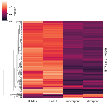
Extended analysis with directional=True

The first analysis presented does not take into account the relative order of TF1-TF2, e.g. if the orientation “same” represents “TF1-TF2” or

[13]:

C.count_within(directional=True, stranded=True, threads=8)
C.market_basket()

[14]:

df = C.analyze_orientation()

INFO: Rules are directional - scenarios counted are: ['TF1-TF2', 'TF2-TF1', 'convergent', 'divergent']

[15]:

df.head()

[15]:

	TF1	TF2	TF1_TF2_count	TF1-TF2	TF2-TF1	convergent	divergent	std	pvalue
SP2-SP2	SP2	SP2	1077	0.395543	0.395543	0.102136	0.106778	0.168069	8.140464e-79
SP1-SP1	SP1	SP1	687	0.417758	0.417758	0.075691	0.088792	0.193784	8.390630e-67
SP3-SP3	SP3	SP3	718	0.412256	0.412256	0.094708	0.080780	0.187444	2.559523e-65
PATZ1-PATZ1	PATZ1	PATZ1	547	0.422303	0.422303	0.078611	0.076782	0.198960	4.875297e-56
SP4-SP4	SP4	SP4	371	0.444744	0.444744	0.070081	0.040431	0.225196	1.132384e-48

Similarly to the first analysis, we can select the significant pairs and visualize the preferences for orientation:

[16]:

selected = df[(df["pvalue"] < 0.05) & (df["TF1_TF2_count"] > 50)]

[17]:

_ = selected.plot_heatmap()

../_images/examples_Orientation_analysis_30_0.png

In-depth look at preferential orientation

By sorting the selected co-occurring TF pairs, it is also possible to visualize the top pairs within each scenario as seen below.

TFs specific in TF1-TF2 orientation

[18]:

selected.sort_values("TF1-TF2", ascending=False).head()

[18]:

	TF1	TF2	TF1_TF2_count	TF1-TF2	TF2-TF1	convergent	divergent	std	pvalue
KLF9-ZNF341	KLF9	ZNF341	80	0.500000	0.337500	0.100000	0.062500	0.206408	6.866468e-09
KLF1-KLF4	KLF1	KLF4	97	0.494845	0.360825	0.041237	0.103093	0.214005	1.575098e-11
KLF4-KLF4	KLF4	KLF4	56	0.482143	0.482143	0.017857	0.017857	0.268055	1.851271e-10
BCL11A-SPIB	BCL11A	SPIB	56	0.482143	0.321429	0.107143	0.089286	0.187287	3.069277e-05
KLF5-ZNF341	KLF5	ZNF341	61	0.475410	0.278689	0.114754	0.131148	0.167382	1.331723e-04

TFs specific in TF2-TF2 orientation

[19]:

selected.sort_values("TF2-TF1", ascending=False).head()

[19]:

	TF1	TF2	TF1_TF2_count	TF1-TF2	TF2-TF1	convergent	divergent	std	pvalue
KLF4-MAZ	KLF4	MAZ	70	0.328571	0.542857	0.042857	0.085714	0.232262	7.933608e-10
EGR1-KLF9	EGR1	KLF9	72	0.277778	0.541667	0.138889	0.041667	0.217248	7.288757e-09
KLF4-KLF5	KLF4	KLF5	63	0.380952	0.539683	0.000000	0.079365	0.253430	1.621951e-10
ETV4-KLF3	ETV4	KLF3	57	0.403509	0.508772	0.017544	0.070175	0.242831	9.055097e-09
E2F6-SP4	E2F6	SP4	80	0.275000	0.500000	0.137500	0.087500	0.184560	3.725792e-07

TFs specific in convergent orientation

[20]:

selected.sort_values("convergent", ascending=False).head()

[20]:

	TF1	TF2	TF1_TF2_count	TF1-TF2	TF2-TF1	convergent	divergent	std	pvalue
ASCL1-SP3	ASCL1	SP3	55	0.127273	0.181818	0.454545	0.236364	0.143452	0.003533
MAZ-ZFX	MAZ	ZFX	54	0.203704	0.111111	0.444444	0.240741	0.140627	0.005055
SP1-ZFX	SP1	ZFX	81	0.111111	0.111111	0.419753	0.358025	0.162343	0.000011
AR-IRF1	AR	IRF1	51	0.274510	0.098039	0.411765	0.215686	0.130433	0.015372
ASCL1-WT1	ASCL1	WT1	61	0.147541	0.114754	0.409836	0.327869	0.141892	0.002055

TFs specific in divergent orientation

[21]:

selected.sort_values("divergent", ascending=False).head()

[21]:

	TF1	TF2	TF1_TF2_count	TF1-TF2	TF2-TF1	convergent	divergent	std	pvalue
STAT2-ZFP28	STAT2	ZFP28	55	0.127273	0.254545	0.181818	0.436364	0.134738	7.445704e-03
KLF3-ZIC3	KLF3	ZIC3	66	0.030303	0.136364	0.409091	0.424242	0.197358	9.148367e-07
IRF3-ZFP28	IRF3	ZFP28	58	0.206897	0.155172	0.224138	0.413793	0.113059	3.069838e-02
NFE2L1-STAT2	NFE2L1	STAT2	68	0.176471	0.220588	0.205882	0.397059	0.099740	4.364185e-02
SP4-ZFX	SP4	ZFX	52	0.192308	0.057692	0.365385	0.384615	0.154645	1.883579e-03