ChIP-seq analysis
This notebook shows how to analyze the TF-co-occurrences of predefined TFBS e.g. from ChIP-seq peaks. The data used here is obtained from the ENCODE project (https://pubmed.ncbi.nlm.nih.gov/29126249/) and consists of all TF ChIP-seq experiments for the celltype GM12878, and subset to chr4 in the human genome.
Setup a CombObj
First, we load the tfcomb package and set up an empty CombObj:
[1]:
from tfcomb import CombObj
C = CombObj()
[2]:
C
[2]:
<CombObj>
Read TFBS from .bed-file
Next, we are going to fill the CombObj ‘C’ with binding sites from GM12878 ChIP-seq experiments:
[3]:
C.TFBS_from_bed("../data/GM12878_hg38_chr4_TF_chipseq.bed")
INFO: Reading sites from '../data/GM12878_hg38_chr4_TF_chipseq.bed'...
INFO: Processing sites
INFO: Read 112109 sites (151 unique names)
Now, the CombObj contains the .TFBS variable holding all TFBS to use for analysis:
[4]:
C.TFBS[:10]
[4]:
[chr4   11875   11876   ZBTB33  1000    .,
 chr4   116639  116640  JUNB    974     .,
 chr4   116678  116679  RUNX3   1000    .,
 chr4   121620  121621  RUNX3   1000    .,
 chr4   124050  124051  ZNF217  948     .,
 chr4   124052  124053  SMARCA5 802     .,
 chr4   124169  124170  NR2F1   634     .,
 chr4   124289  124290  CBX5    906     .,
 chr4   124363  124364  E4F1    1000    .,
 chr4   124365  124366  PKNOX1  1000    .]
The CombObj will now reflect that TFBS were added:
[5]:
C
[5]:
<CombObj: 112109 TFBS (151 unique names)>
Perform market basket analysis
Next, the function .market_basket() is used to perform the co-occurrence analysis of the sites just added to .TFBS:
[6]:
C.market_basket()
Internal counts for 'TF_counts' were not set. Please run .count_within() to obtain TF-TF co-occurrence counts.
WARNING: No counts found in <CombObj>. Running <CombObj>.count_within() with standard parameters.
INFO: Setting up binding sites for counting
INFO: Counting co-occurrences within sites
INFO: Counting co-occurrence within background
INFO: Running with multiprocessing threads == 1. To change this, give 'threads' in the parameter of the function.
INFO: Progress: 10%
INFO: Progress: 20%
INFO: Progress: 30%
INFO: Progress: 40%
INFO: Progress: 50%
INFO: Progress: 60%
INFO: Progress: 70%
INFO: Progress: 80%
INFO: Progress: 90%
INFO: Done finding co-occurrences! Run .market_basket() to estimate significant pairs
INFO: Market basket analysis is done! Results are found in <CombObj>.rules
As is shown in the info messages, this also runs the .count_within() function of ‘C’ (if no counts were found yet). If you want to set specific parameters for count_within, you can split these calculations such as seen here:
C.count_within(max_distance=200)
C.market_basket()
In any case, running .market_basket() will fill out the .rules variable of the CombObj:
[7]:
C.rules.head()
[7]:
| TF1 | TF2 | TF1_TF2_count | TF1_count | TF2_count | cosine | zscore | |
|---|---|---|---|---|---|---|---|
| CTCF-RAD21 | CTCF | RAD21 | 1751 | 2432 | 2241 | 0.750038 | 18.643056 |
| RAD21-CTCF | RAD21 | CTCF | 1751 | 2241 | 2432 | 0.750038 | 18.643056 |
| RAD21-SMC3 | RAD21 | SMC3 | 1376 | 2241 | 1638 | 0.718192 | 20.314026 |
| SMC3-RAD21 | SMC3 | RAD21 | 1376 | 1638 | 2241 | 0.718192 | 20.314026 |
| CTCF-SMC3 | CTCF | SMC3 | 1361 | 2432 | 1638 | 0.681898 | 20.245177 |
Printing the CombObj again will also tell you how many rules were found in the market basket analysis:
[8]:
C
[8]:
<CombObj: 112109 TFBS (151 unique names) | Market basket analysis: 21284 rules>
Visualize results
The CombObj ‘C’ contains a number of different visualizations for the identified TF-TF co-occurrence pairs. The default measure plotted is ‘cosine’, but many of the options of the plots can be changed as seen in the examples below:
Heatmap
[9]:
_ = C.plot_heatmap()

[10]:
#Showing more rules
_ = C.plot_heatmap(n_rules=50)

[11]:
#Coloring the heatmap by TF1_TF2_count
_ = C.plot_heatmap(color_by="TF1_TF2_count")

Bubble plot
[12]:
_ = C.plot_bubble()
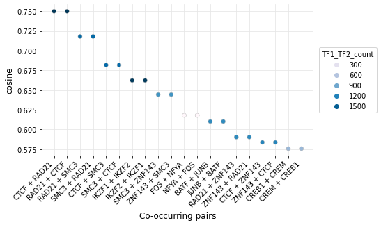
[13]:
#Show more rules
_ = C.plot_bubble(n_rules=40, figsize=(12,4))

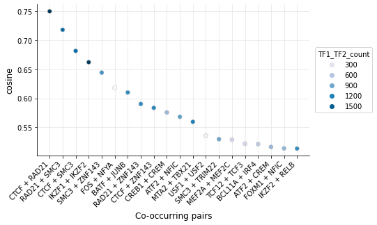
Handling duplicate rules
As seen in the bubble plot above, the rules are duplicated due to the cosine measure, which scores TF1-TF2 the same way as TF2-TF1. In order to simplify the results, you can use .simplify_rules() to remove the duplicates from the .rules:
[14]:
C.simplify_rules()
[15]:
C.rules
[15]:
| TF1 | TF2 | TF1_TF2_count | TF1_count | TF2_count | cosine | zscore | |
|---|---|---|---|---|---|---|---|
| CTCF-RAD21 | CTCF | RAD21 | 1751 | 2432 | 2241 | 0.750038 | 18.643056 |
| RAD21-SMC3 | RAD21 | SMC3 | 1376 | 2241 | 1638 | 0.718192 | 20.314026 |
| CTCF-SMC3 | CTCF | SMC3 | 1361 | 2432 | 1638 | 0.681898 | 20.245177 |
| IKZF1-IKZF2 | IKZF1 | IKZF2 | 1726 | 2922 | 2324 | 0.662343 | 11.215960 |
| SMC3-ZNF143 | SMC3 | ZNF143 | 1060 | 1638 | 1652 | 0.644383 | 21.838431 |
| ... | ... | ... | ... | ... | ... | ... | ... |
| HDAC6-JUNB | HDAC6 | JUNB | 1 | 172 | 1866 | 0.001765 | -6.905016 |
| RELB-SUZ12 | RELB | SUZ12 | 1 | 2011 | 172 | 0.001700 | -6.793962 |
| ATF7-SUZ12 | ATF7 | SUZ12 | 1 | 2061 | 172 | 0.001680 | -6.119294 |
| RAD21-SUZ12 | RAD21 | SUZ12 | 1 | 2241 | 172 | 0.001611 | -7.500216 |
| IKZF2-SUZ12 | IKZF2 | SUZ12 | 1 | 2324 | 172 | 0.001582 | -6.649424 |
10642 rows × 7 columns
Now, you can again use plot_bubble() to visualize the highest-scoring co-occurring pairs:
[16]:
_ = C.plot_bubble()
Save CombObj to a pickle object
We can now save the CombObj to a pickle object to be used in other analysis:
[17]:
C.to_pickle("../data/GM12878.pkl")