Binding distance analysis
For more details on how to perform the market basket step please have a look at the TFBS from motif or ChIP-seq analysis examples.
Content:
Prepare object
-
Create object
Count distances
Smoothing counts
Scale counts
Correct background
Analyse signal
z-score
Flat
-
Analyzing hubs
Signal classification
Prepare a CombObj
[1]:
import tfcomb.objects

C = tfcomb.objects.CombObj()
C.TFBS_from_motifs(regions="../data/GM12878_hg38_chr4_ATAC_peaks.bed",
                   motifs="../data/HOCOMOCOv11_HUMAN_motifs.txt",
                   genome="../data/hg38_chr4.fa.gz",
                   threads=4)
C.count_within(max_overlap=0.0, threads=4)
C.market_basket()
C.rules.head()
INFO: Scanning for TFBS with 4 thread(s)...
INFO: Progress: 11%
INFO: Progress: 20%
INFO: Progress: 30%
INFO: Progress: 40%
INFO: Progress: 50%
INFO: Progress: 60%
INFO: Progress: 71%
INFO: Progress: 82%
INFO: Progress: 91%
INFO: Finished!
INFO: Processing scanned TFBS
INFO: Identified 165810 TFBS (401 unique names) within given regions
INFO: Setting up binding sites for counting
INFO: Counting co-occurrences within sites
INFO: Counting co-occurrence within background
INFO: Progress: 16%
INFO: Progress: 20%
INFO: Progress: 32%
INFO: Progress: 40%
INFO: Progress: 50%
INFO: Progress: 62%
INFO: Progress: 72%
INFO: Progress: 80%
INFO: Progress: 92%
INFO: Finished!
INFO: Done finding co-occurrences! Run .market_basket() to estimate significant pairs
INFO: Market basket analysis is done! Results are found in <CombObj>.rules
[1]:
| TF1 | TF2 | TF1_TF2_count | TF1_count | TF2_count | cosine | zscore | |
|---|---|---|---|---|---|---|---|
| POU3F2-SMARCA5 | POU3F2 | SMARCA5 | 239 | 302 | 241 | 0.885902 | 129.586528 |
| SMARCA5-POU3F2 | SMARCA5 | POU3F2 | 239 | 241 | 302 | 0.885902 | 129.586528 |
| POU2F1-SMARCA5 | POU2F1 | SMARCA5 | 263 | 426 | 241 | 0.820810 | 135.355691 |
| SMARCA5-POU2F1 | SMARCA5 | POU2F1 | 263 | 241 | 426 | 0.820810 | 135.355691 |
| SMARCA5-ZNF582 | SMARCA5 | ZNF582 | 172 | 241 | 195 | 0.793419 | 117.370387 |
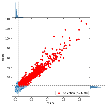
Selecting rules
[2]:
selection = C.select_significant_rules()
INFO: x_threshold is None; trying to calculate optimal threshold
INFO: y_threshold is None; trying to calculate optimal threshold
INFO: Creating subset of TFBS and rules using thresholds
Method 1: Automated analysis
There are two different ways to run this analysis. The automated way will be shown in this chapter. Followed by an in depth guide showing the analysis step by step in the next chapter.
Here we will start with the automated analysis for all selected rules.
[3]:
selection.analyze_distances(threads=6) # adjust threads if needed
INFO: DistObject successfully created! It can be accessed via <CombObj>.distObj
INFO: Preparing to count distances.
INFO: Setting up binding sites for counting
INFO: Calculating distances
INFO: Done finding distances! Results are found in .distances
INFO: You can now run .smooth() and/or .correct_background() to preprocess sites before finding peaks.
INFO: Or you can find peaks directly using .analyze_signal_all()
INFO: Smoothing signals with window size 3
INFO: Background correction finished! Results can be found in .corrected
INFO: Analyzing Signal with threads 6
INFO: Calculating zscores for signals
INFO: Finding preferred distances
INFO: Done analyzing signal. Results are found in .peaks
[4]:
selection.distObj.peaks.loc[(selection.distObj.peaks.TF1 == "ZNF121") & (selection.distObj.peaks.TF2 == "ZNF770")]
[4]:
| TF1 | TF2 | Distance | Peak Heights | Prominences | Threshold | TF1_TF2_count | Distance_count | Distance_percent | Distance_window | |
|---|---|---|---|---|---|---|---|---|---|---|
| ZNF121-ZNF770 | ZNF121 | ZNF770 | 26 | 4.043651 | 4.443567 | 2 | 1319 | 381 | 28.885519 | [25;27] |
| ZNF121-ZNF770 | ZNF121 | ZNF770 | 58 | 3.906961 | 4.353073 | 2 | 1319 | 376 | 28.506444 | [57;59] |
| ZNF121-ZNF770 | ZNF121 | ZNF770 | 66 | 2.068096 | 2.270661 | 2 | 1319 | 220 | 16.679303 | [65;67] |
[5]:
_ = selection.distObj.plot(("ZNF121", "ZNF770"))

On the x-axis the distance in bp is shown. For example a distance of 100 means the anchors (depending on anchor mode, please refer to Anchor mode on this topic) are 100 bp away of each other. On the y-axis of the plot the calculated zscore per distance is shown.
For an explaination of the results please refer to the in depth guide below.
Method 2: Step-by-Step Analysis
Besides the automated way, the analysis can be done step-by-step. This chapter is an detailed guide, covering all 5 major steps.
1. Create a distance object
The binding distance analysis can be started from within any combObj. In this example the appropiate object is called selection, since we only want to use significant rules, not all. The analysis can also be done without pre selection.
[6]:
selection.create_distObj()
INFO: DistObject successfully created! It can be accessed via <CombObj>.distObj
As stated in the information message, the distObj should be created successfully and filled with all important information to start the distance analysis. This includes parameters set for the market masket analysis.
[7]:
selection.distObj
[7]:
<tfcomb.objects.DistObj at 0x7f87d1e6a950>
The 3792 rules (market basket results) selected earlier by select.significant_rules() are automatically passed to the distance object during creation:
[8]:
selection.distObj.rules
[8]:
| TF1 | TF2 | TF1_TF2_count | TF1_count | TF2_count | cosine | zscore | |
|---|---|---|---|---|---|---|---|
| POU3F2-SMARCA5 | POU3F2 | SMARCA5 | 239 | 302 | 241 | 0.885902 | 129.586528 |
| SMARCA5-POU3F2 | SMARCA5 | POU3F2 | 239 | 241 | 302 | 0.885902 | 129.586528 |
| POU2F1-SMARCA5 | POU2F1 | SMARCA5 | 263 | 426 | 241 | 0.820810 | 135.355691 |
| SMARCA5-POU2F1 | SMARCA5 | POU2F1 | 263 | 241 | 426 | 0.820810 | 135.355691 |
| SMARCA5-ZNF582 | SMARCA5 | ZNF582 | 172 | 241 | 195 | 0.793419 | 117.370387 |
| ... | ... | ... | ... | ... | ... | ... | ... |
| NFYB-EGR2 | NFYB | EGR2 | 24 | 219 | 1304 | 0.044911 | 3.401991 |
| MYOG-TAF1 | MYOG | TAF1 | 23 | 386 | 681 | 0.044860 | 3.375730 |
| TAF1-MYOG | TAF1 | MYOG | 23 | 681 | 386 | 0.044860 | 3.375730 |
| ETV1-ZBTB17 | ETV1 | ZBTB17 | 20 | 117 | 1699 | 0.044858 | 3.064184 |
| ZBTB17-ETV1 | ZBTB17 | ETV1 | 20 | 1699 | 117 | 0.044858 | 3.064184 |
3778 rows × 7 columns
will be set automatically when creating the distance object according to the values used for the market basket analysis step.
[9]:
selection.distObj.max_overlap
[9]:
0.0
2. Distance counting
After creating the distObj, the first step is to count the distances. This will be done with .count_distances(). In this step it is important to decide if the directionality should be taken into account.
If directionality is taken into account the position of the transcription factors do matter. This means there is a difference between TFA -> TFB and TFB -> TFA (compare Orientation analysis notebook). Otherwise TFA -> TFB and TFB -> TFA are the same.
Per default the directionality decision is copied from the market basket step.
[10]:
selection.distObj.directional
[10]:
False
[11]:
selection.distObj.count_distances()
INFO: Preparing to count distances.
INFO: Setting up binding sites for counting
INFO: Calculating distances
INFO: Done finding distances! Results are found in .distances
INFO: You can now run .smooth() and/or .correct_background() to preprocess sites before finding peaks.
INFO: Or you can find peaks directly using .analyze_signal_all()
The resulting dataframe is constructed as followed: - columns: First the transcription factor for the pair (TF1, TF2) followed by the distances in bp - rows: each row representing one rule (pair) with the corresponding results
[12]:
selection.distObj.distances
[12]:
| TF1 | TF2 | 0 | 1 | 2 | 3 | 4 | 5 | 6 | 7 | ... | 91 | 92 | 93 | 94 | 95 | 96 | 97 | 98 | 99 | 100 | |
|---|---|---|---|---|---|---|---|---|---|---|---|---|---|---|---|---|---|---|---|---|---|
| POU3F2-SMARCA5 | POU3F2 | SMARCA5 | 2 | 0 | 0 | 7 | 0 | 15 | 0 | 1 | ... | 0 | 0 | 7 | 1 | 6 | 0 | 0 | 3 | 0 | 3 |
| SMARCA5-POU3F2 | SMARCA5 | POU3F2 | 2 | 0 | 0 | 7 | 0 | 15 | 0 | 1 | ... | 0 | 0 | 7 | 1 | 6 | 0 | 0 | 3 | 0 | 3 |
| POU2F1-SMARCA5 | POU2F1 | SMARCA5 | 0 | 2 | 0 | 39 | 0 | 0 | 12 | 1 | ... | 4 | 0 | 5 | 0 | 0 | 4 | 0 | 1 | 0 | 1 |
| SMARCA5-POU2F1 | SMARCA5 | POU2F1 | 0 | 2 | 0 | 39 | 0 | 0 | 12 | 1 | ... | 4 | 0 | 5 | 0 | 0 | 4 | 0 | 1 | 0 | 1 |
| SMARCA5-ZNF582 | SMARCA5 | ZNF582 | 0 | 0 | 38 | 0 | 36 | 1 | 1 | 2 | ... | 0 | 4 | 0 | 2 | 0 | 0 | 2 | 0 | 1 | 0 |
| ... | ... | ... | ... | ... | ... | ... | ... | ... | ... | ... | ... | ... | ... | ... | ... | ... | ... | ... | ... | ... | ... |
| NFYB-EGR2 | NFYB | EGR2 | 2 | 0 | 1 | 0 | 0 | 0 | 1 | 0 | ... | 0 | 0 | 0 | 0 | 0 | 0 | 1 | 0 | 0 | 0 |
| MYOG-TAF1 | MYOG | TAF1 | 0 | 1 | 1 | 0 | 1 | 0 | 0 | 0 | ... | 0 | 0 | 0 | 0 | 0 | 0 | 0 | 0 | 1 | 0 |
| TAF1-MYOG | TAF1 | MYOG | 0 | 1 | 1 | 0 | 1 | 0 | 0 | 0 | ... | 0 | 0 | 0 | 0 | 0 | 0 | 0 | 0 | 1 | 0 |
| ETV1-ZBTB17 | ETV1 | ZBTB17 | 0 | 0 | 0 | 0 | 0 | 0 | 1 | 1 | ... | 0 | 0 | 0 | 1 | 1 | 0 | 1 | 0 | 0 | 0 |
| ZBTB17-ETV1 | ZBTB17 | ETV1 | 0 | 0 | 0 | 0 | 0 | 0 | 1 | 1 | ... | 0 | 0 | 0 | 1 | 1 | 0 | 1 | 0 | 0 | 0 |
3778 rows × 103 columns
Additional options for counting distances
Negative distances
Anchor mode
TFCOMB distance analysis supports three different anchor modes: inner , outer and center. The recommended mode is inner.
inner (default, recommented) is the distance between the transcription factors, it is measures as start(transcription factor B) - end(transcription factor A). If for example transcription factor B is directly adjacent to Transcription factor A, the difference will be zero.
center is the distance measured from mid of transcription factor to mid of transcription factor
outer (uncommonly used) is the distance measured including both transcription factors. end(transcription factor B) - start(transcription factor A)
Directionality
Since we didn’t count directional, the values for the pairs TF1-TF2 and TF2-TF1 should be equal. For example in the DataFrame above the results for ZNF121-ZNF770 are the same as for ZNF770-ZNF121. This is not true if directionality is considered.
Note: If directionality is not considered, the duplicates can be filtered with .simplify_rules()
Plotting
There are different ways to plot the distance distribution, you can for example create a kernel density estimate (KDE) plot or a histogram of the distribution.
[13]:
selection.distObj.plot(("ZNF121", "ZNF770"), style="kde")
[13]:
<AxesSubplot:title={'center':'ZNF121-ZNF770'}, xlabel='Distance (bp)', ylabel='Count per distance'>

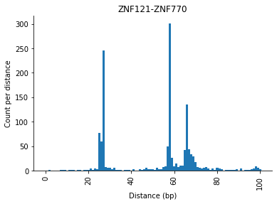
[14]:
selection.distObj.plot(("ZNF121", "ZNF770"), style="hist")
[14]:
<AxesSubplot:title={'center':'ZNF121-ZNF770'}, xlabel='Distance (bp)', ylabel='Count per distance'>
3. Smoothing counts
In order to collect distances from more than one basepair, e.g. in a window, it is possible to smooth the counted distances. This is done using the function .smooth() of the distObj:
[15]:
selection.distObj.smooth(window_size=3)
INFO: Smoothing signals with window size 3
The smoothed (min-max-scaled) distances are visible in the .smoothed variable:
[16]:
selection.distObj.smoothed.head()
[16]:
| TF1 | TF2 | 1 | 2 | 3 | 4 | 5 | 6 | 7 | 8 | ... | 90 | 91 | 92 | 93 | 94 | 95 | 96 | 97 | 98 | 99 | |
|---|---|---|---|---|---|---|---|---|---|---|---|---|---|---|---|---|---|---|---|---|---|
| POU3F2-SMARCA5 | POU3F2 | SMARCA5 | 0.666667 | 2.333333 | 2.333333 | 7.333333 | 5.000000 | 5.333333 | 10.333333 | 10.333333 | ... | 1.666667 | 1.666667 | 2.333333 | 2.666667 | 4.666667 | 2.333333 | 2.000000 | 1.000000 | 1.000000 | 2.000000 |
| SMARCA5-POU3F2 | SMARCA5 | POU3F2 | 0.666667 | 2.333333 | 2.333333 | 7.333333 | 5.000000 | 5.333333 | 10.333333 | 10.333333 | ... | 1.666667 | 1.666667 | 2.333333 | 2.666667 | 4.666667 | 2.333333 | 2.000000 | 1.000000 | 1.000000 | 2.000000 |
| POU2F1-SMARCA5 | POU2F1 | SMARCA5 | 0.666667 | 13.666667 | 13.000000 | 13.000000 | 4.000000 | 4.333333 | 5.333333 | 1.333333 | ... | 1.333333 | 1.333333 | 3.000000 | 1.666667 | 1.666667 | 1.333333 | 1.333333 | 1.666667 | 0.333333 | 0.666667 |
| SMARCA5-POU2F1 | SMARCA5 | POU2F1 | 0.666667 | 13.666667 | 13.000000 | 13.000000 | 4.000000 | 4.333333 | 5.333333 | 1.333333 | ... | 1.333333 | 1.333333 | 3.000000 | 1.666667 | 1.666667 | 1.333333 | 1.333333 | 1.666667 | 0.333333 | 0.666667 |
| SMARCA5-ZNF582 | SMARCA5 | ZNF582 | 12.666667 | 12.666667 | 24.666667 | 12.333333 | 12.666667 | 1.333333 | 1.333333 | 3.333333 | ... | 1.333333 | 1.333333 | 1.333333 | 2.000000 | 0.666667 | 0.666667 | 0.666667 | 0.666667 | 1.000000 | 0.333333 |
5 rows × 101 columns
4. Scale counts (optional)
Optionally, it is possible to scale the counts to be in the same ranges regardless of number of counts per pair.
[17]:
selection_copy = selection.copy() #create a copy to not alter the real selection object
selection_copy.distObj.scale()
[18]:
selection_copy.distObj.scaled.head()
[18]:
| TF1 | TF2 | 1 | 2 | 3 | 4 | 5 | 6 | 7 | 8 | ... | 90 | 91 | 92 | 93 | 94 | 95 | 96 | 97 | 98 | 99 | |
|---|---|---|---|---|---|---|---|---|---|---|---|---|---|---|---|---|---|---|---|---|---|
| POU3F2-SMARCA5 | POU3F2 | SMARCA5 | 0.017857 | 0.107143 | 0.107143 | 0.375 | 0.250000 | 0.267857 | 0.535714 | 0.535714 | ... | 0.071429 | 0.071429 | 0.107143 | 0.125000 | 0.232143 | 0.107143 | 0.089286 | 0.035714 | 0.035714 | 0.089286 |
| SMARCA5-POU3F2 | SMARCA5 | POU3F2 | 0.017857 | 0.107143 | 0.107143 | 0.375 | 0.250000 | 0.267857 | 0.535714 | 0.535714 | ... | 0.071429 | 0.071429 | 0.107143 | 0.125000 | 0.232143 | 0.107143 | 0.089286 | 0.035714 | 0.035714 | 0.089286 |
| POU2F1-SMARCA5 | POU2F1 | SMARCA5 | 0.025000 | 1.000000 | 0.950000 | 0.950 | 0.275000 | 0.300000 | 0.375000 | 0.075000 | ... | 0.075000 | 0.075000 | 0.200000 | 0.100000 | 0.100000 | 0.075000 | 0.075000 | 0.100000 | 0.000000 | 0.025000 |
| SMARCA5-POU2F1 | SMARCA5 | POU2F1 | 0.025000 | 1.000000 | 0.950000 | 0.950 | 0.275000 | 0.300000 | 0.375000 | 0.075000 | ... | 0.075000 | 0.075000 | 0.200000 | 0.100000 | 0.100000 | 0.075000 | 0.075000 | 0.100000 | 0.000000 | 0.025000 |
| SMARCA5-ZNF582 | SMARCA5 | ZNF582 | 0.513514 | 0.513514 | 1.000000 | 0.500 | 0.513514 | 0.054054 | 0.054054 | 0.135135 | ... | 0.054054 | 0.054054 | 0.054054 | 0.081081 | 0.027027 | 0.027027 | 0.027027 | 0.027027 | 0.040541 | 0.013514 |
5 rows × 101 columns
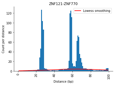
5. Background correction
To separate the signal from the background noise a linear regression for every signal needs to be fitted next. The result of the fitted line for every pair can be found in the .linres attribute of the distance object.
[19]:
selection.distObj.correct_background(threads=6)
INFO: Background correction finished! Results can be found in .corrected
The fitted lowess function can be plotted with the .plot() command. The red line indicates the linear regression line which was fitted during this step.
[20]:
_ = selection.distObj.plot(("ZNF121", "ZNF770"), method="correction")
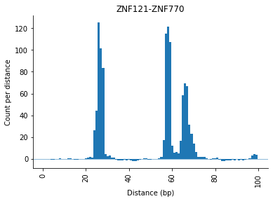
After correction, the plotting function will show the corrected counts:
[21]:
_ = selection.distObj.plot(("ZNF121", "ZNF770"))
6. Analyse signal
As a last step, the corrected signal can now be analyzed. Peaks will be called with *scipy.signal.find_peaks()*. Two different methods are available:
“zscore”
“flat” (number)
Zscore method
If prominence is set to zscore, the threshold is set in relation to the zscore (of the corrected signal) for each signal. For example if threshold is 2, the threshold prominence (for the score translated signal) will be a zscore of two.
[22]:
selection.distObj.analyze_signal_all(method="zscore", threshold=2, threads=6)
selection.distObj.peaks
INFO: Analyzing Signal with threads 6
INFO: Calculating zscores for signals
INFO: Finding preferred distances
INFO: Done analyzing signal. Results are found in .peaks
[22]:
| TF1 | TF2 | Distance | Peak Heights | Prominences | Threshold | TF1_TF2_count | Distance_count | Distance_percent | Distance_window | |
|---|---|---|---|---|---|---|---|---|---|---|
| ZFP82-SMARCA5 | ZFP82 | SMARCA5 | 8 | 6.547058 | 7.582435 | 2 | 198 | 46 | 23.232323 | [7;9] |
| SMARCA5-ZFP82 | SMARCA5 | ZFP82 | 8 | 6.547058 | 7.582435 | 2 | 198 | 46 | 23.232323 | [7;9] |
| ZNF394-SMARCA5 | ZNF394 | SMARCA5 | 5 | 6.940786 | 7.474373 | 2 | 187 | 74 | 39.572193 | [4;6] |
| SMARCA5-ZNF394 | SMARCA5 | ZNF394 | 5 | 6.940786 | 7.474373 | 2 | 187 | 74 | 39.572193 | [4;6] |
| POU3F2-SMARCA5 | POU3F2 | SMARCA5 | 9 | 6.584317 | 7.402690 | 2 | 234 | 57 | 24.358974 | [8;10] |
| ... | ... | ... | ... | ... | ... | ... | ... | ... | ... | ... |
| ETV5-ZSCAN22 | ETV5 | ZSCAN22 | 98 | 2.010752 | 2.010752 | 2 | 64 | 3 | 4.687500 | [97;99] |
| ZBTB17-RFX1 | ZBTB17 | RFX1 | 1 | 2.010639 | 2.010639 | 2 | 30 | 1 | 3.333333 | [1;2] |
| RFX1-ZBTB17 | RFX1 | ZBTB17 | 1 | 2.010639 | 2.010639 | 2 | 30 | 1 | 3.333333 | [1;2] |
| WT1-ZIC3 | WT1 | ZIC3 | 48 | 2.226574 | 2.005542 | 2 | 51 | 4 | 7.843137 | [47;49] |
| ZIC3-WT1 | ZIC3 | WT1 | 48 | 2.226574 | 2.005542 | 2 | 51 | 4 | 7.843137 | [47;49] |
8160 rows × 10 columns
The resulting dataframe is constructed as followed: - columns: First the transcription factor for the pair (TF1, TF2) followed by
1. __Distance__ in bp \
2. __Peak Heights__ height of the peak (calculated by [_find_peaks()_](https://docs.scipy.org/doc/scipy/reference/generated/scipy.signal.find_peaks.html)). \
3. __Prominences__ prominence of the peak (calculated by [_find_peaks()_](https://docs.scipy.org/doc/scipy/reference/generated/scipy.signal.find_peaks.html)). \
4. __Threshold__ minimum prominence needed to be considered as peak (in this example the [zscore](#5.B.-Zscore) of the signal). \
5. __TF1_TF2_count__ is the total number of co-occurring TF1-TF2 sites. \
6. __Distance_count__ The number of co-occurrences for the given distance. \
7. __Distance_percent__ The percent of Distance_count of the total sites (TF1_TF2_count). \
8. __Distance_window__ The distances collected for the given distance. Will be a window if smoothing was applied. \
rows: each row representing one rule (pair) at a distinct prefered binding distance with the corresponding results
The signal and peaks can now be plotted with the .plot() command.
[23]:
selection.distObj.plot(("ZNF121", "ZNF770"))
[23]:
<AxesSubplot:title={'center':'ZNF121-ZNF770'}, xlabel='Distance (bp)', ylabel='Z-score normalized counts'>

This plot shows the corrected signal with the called peaks, indicated by a cross.
The grey dottet line shows the decision boundary (in this example a zscore of 2)
[24]:
selection.distObj.peaks.loc[(selection.distObj.peaks.TF1 == "ZNF121") & (selection.distObj.peaks.TF2 == "ZNF770")]
[24]:
| TF1 | TF2 | Distance | Peak Heights | Prominences | Threshold | TF1_TF2_count | Distance_count | Distance_percent | Distance_window | |
|---|---|---|---|---|---|---|---|---|---|---|
| ZNF121-ZNF770 | ZNF121 | ZNF770 | 26 | 4.043651 | 4.443567 | 2 | 1319 | 381 | 28.885519 | [25;27] |
| ZNF121-ZNF770 | ZNF121 | ZNF770 | 58 | 3.906961 | 4.353073 | 2 | 1319 | 376 | 28.506444 | [57;59] |
| ZNF121-ZNF770 | ZNF121 | ZNF770 | 66 | 2.068096 | 2.270661 | 2 | 1319 | 220 | 16.679303 | [65;67] |
The results in the .peaks table and the plot matches. For this ZNF121-ZNF770 3 peaks were found, which also can be seen in the plot at positions:
distance: 26
distance: 58
distance: 66
Meaning the zscore threshold with stringency of 2 identifies 3 different preferred distances for this pair. Please note, that the height of the distances differ!
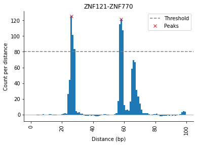
#### Flat threshold
Using a flat threshold, it is possible to only find peaks with a certain number of counts as seen here:
[25]:
selection.distObj.analyze_signal_all(method="flat", threshold=80, threads=6)
selection.distObj.peaks
INFO: Analyzing Signal with threads 6
INFO: Calculating zscores for signals
INFO: Finding preferred distances
INFO: Done analyzing signal. Results are found in .peaks
[25]:
| TF1 | TF2 | Distance | Peak Heights | Prominences | Threshold | TF1_TF2_count | Distance_count | Distance_percent | Distance_window | |
|---|---|---|---|---|---|---|---|---|---|---|
| ZNF121-ZNF770 | ZNF121 | ZNF770 | 26 | 125.175641 | 125.839985 | 80 | 1319 | 381 | 28.885519 | [25;27] |
| ZNF770-ZNF121 | ZNF770 | ZNF121 | 26 | 125.175641 | 125.839985 | 80 | 1319 | 381 | 28.885519 | [25;27] |
| ZNF121-ZNF770 | ZNF121 | ZNF770 | 58 | 121.304647 | 123.277229 | 80 | 1319 | 376 | 28.506444 | [57;59] |
| ZNF770-ZNF121 | ZNF770 | ZNF121 | 58 | 121.304647 | 123.277229 | 80 | 1319 | 376 | 28.506444 | [57;59] |
| PAX5-ZNF770 | PAX5 | ZNF770 | 56 | 104.564327 | 106.526327 | 80 | 896 | 325 | 36.272321 | [55;57] |
| ZNF770-PAX5 | ZNF770 | PAX5 | 56 | 104.564327 | 106.526327 | 80 | 896 | 325 | 36.272321 | [55;57] |
[26]:
selection.distObj.plot(("ZNF121", "ZNF770"))
[26]:
<AxesSubplot:title={'center':'ZNF121-ZNF770'}, xlabel='Distance (bp)', ylabel='Count per distance'>
Further downstream analysis
1. Analyzing hubs
This function allows to summarize the number of different partners (with at least one peak) each transcription factor has.
[27]:
selection.distObj.analyze_hubs().sort_values()
[27]:
PAX5      1
ZNF121    1
ZNF770    2
dtype: int64
2. Signal classification
This function allows to classify the pairs (in .distance DataFrame) wheather the signal is peaking or not.
[28]:
selection.distObj.classify_rules()
selection.distObj.classified.sort_values(by="isPeaking")
INFO: classifying rules
INFO: classifcation done. Results can be found in .classified
[28]:
| TF1 | TF2 | isPeaking | |
|---|---|---|---|
| POU3F2-SMARCA5 | POU3F2 | SMARCA5 | False |
| ELK4-WT1 | ELK4 | WT1 | False |
| WT1-ELK4 | WT1 | ELK4 | False |
| ELF2-SP1 | ELF2 | SP1 | False |
| SP1-ELF2 | SP1 | ELF2 | False |
| ... | ... | ... | ... |
| ZBTB17-ETV1 | ZBTB17 | ETV1 | False |
| ZNF121-ZNF770 | ZNF121 | ZNF770 | True |
| PAX5-ZNF770 | PAX5 | ZNF770 | True |
| ZNF770-PAX5 | ZNF770 | PAX5 | True |
| ZNF770-ZNF121 | ZNF770 | ZNF121 | True |
3778 rows × 3 columns
True means the signal has at least one peak found, False otherwise.