TFBS from motifs
In this notebook, we show how a CombObj can be set up using motifs and a set of target regions.
Setup a CombObj
[1]:
from tfcomb import CombObj
C = CombObj()
Search for TFBS within peak regions
We are using a subset of ATAC-seq peaks from GM12878 as the target regions. The .TFBS variable can then be filled as seen here:
[2]:
C.TFBS_from_motifs(regions="../data/GM12878_hg38_chr4_ATAC_peaks.bed",
                   motifs="../data/HOCOMOCOv11_HUMAN_motifs.txt",
                   genome="../data/hg38_chr4.fa.gz",
                   threads=4)
INFO: Scanning for TFBS with 4 thread(s)...
INFO: Progress: 11%
INFO: Progress: 20%
INFO: Progress: 30%
INFO: Progress: 41%
INFO: Progress: 50%
INFO: Progress: 60%
INFO: Progress: 70%
INFO: Progress: 81%
INFO: Progress: 90%
INFO: Finished!
INFO: Processing scanned TFBS
INFO: Identified 165810 TFBS (401 unique names) within given regions
[3]:
C.TFBS[:10]
[3]:
[chr4   11750   11772   THAP1   10.09272        +,
 chr4   11806   11823   CTCFL   12.12093        -,
 chr4   11806   11825   CTCF    13.68703        -,
 chr4   11864   11881   CTCFL   12.23068        -,
 chr4   11864   11883   CTCF    12.56734        -,
 chr4   11938   11945   MYF6    8.75866 -,
 chr4   11997   12010   MYOG    9.91354 -,
 chr4   11999   12009   TCF12   9.23823 +,
 chr4   11999   12009   TCF4    9.99356 +,
 chr4   12000   12007   MYF6    8.75866 -]
Perform market basket analysis
As shown in previous notebooks, we can now perform the market basket analysis on the sites within .TFBS:
[4]:
C.market_basket(threads=10)
Internal counts for 'TF_counts' were not set. Please run .count_within() to obtain TF-TF co-occurrence counts.
WARNING: No counts found in <CombObj>. Running <CombObj>.count_within() with standard parameters.
INFO: Setting up binding sites for counting
INFO: Counting co-occurrences within sites
INFO: Counting co-occurrence within background
INFO: Progress: 14%
INFO: Progress: 28%
INFO: Progress: 40%
INFO: Progress: 52%
INFO: Progress: 64%
INFO: Progress: 76%
INFO: Progress: 88%
INFO: Finished!
INFO: Done finding co-occurrences! Run .market_basket() to estimate significant pairs
INFO: Market basket analysis is done! Results are found in <CombObj>.rules
[5]:
C
[5]:
<CombObj: 165810 TFBS (401 unique names) | Market basket analysis: 126997 rules>
[6]:
C.rules.head()
[6]:
| TF1 | TF2 | TF1_TF2_count | TF1_count | TF2_count | cosine | zscore | |
|---|---|---|---|---|---|---|---|
| POU3F2-SMARCA5 | POU3F2 | SMARCA5 | 239 | 302 | 241 | 0.885902 | 129.586528 |
| SMARCA5-POU3F2 | SMARCA5 | POU3F2 | 239 | 241 | 302 | 0.885902 | 129.586528 |
| POU2F1-SMARCA5 | POU2F1 | SMARCA5 | 263 | 426 | 241 | 0.820810 | 135.355691 |
| SMARCA5-POU2F1 | SMARCA5 | POU2F1 | 263 | 241 | 426 | 0.820810 | 135.355691 |
| SMARCA5-ZNF582 | SMARCA5 | ZNF582 | 172 | 241 | 195 | 0.793419 | 117.370387 |
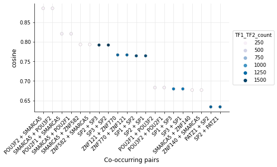
Visualize rules
With the market basket analysis done, we have the option to visualize the identified co-occurring TFs:
[7]:
_ = C.plot_heatmap()

[8]:
_ = C.plot_bubble()
The effect of count parameters
In this example, the first rules contain more TF1_TF2_counts than the individual counts of TF1 and TF2:
[9]:
C.rules.head(1)
[9]:
| TF1 | TF2 | TF1_TF2_count | TF1_count | TF2_count | cosine | zscore | |
|---|---|---|---|---|---|---|---|
| POU3F2-SMARCA5 | POU3F2 | SMARCA5 | 239 | 302 | 241 | 0.885902 | 129.586528 |
How can that be? If there are multiple combinations of TF1-TF2 within the same window, these combinations can add up to more than the number of individual TF positions. This effect can be controlled by setting binarize=True in count_within. This will ensure that each co-occurrence is only counted once per window:
[10]:
C.count_within(binarize=True, threads=8)
C.market_basket()
INFO: Counting co-occurrences within sites
INFO: Counting co-occurrence within background
INFO: Progress: 16%
INFO: Progress: 28%
INFO: Progress: 32%
INFO: Progress: 44%
INFO: Progress: 54%
INFO: Progress: 64%
INFO: Progress: 72%
INFO: Progress: 80%
INFO: Progress: 92%
INFO: Finished!
INFO: Done finding co-occurrences! Run .market_basket() to estimate significant pairs
INFO: Market basket analysis is done! Results are found in <CombObj>.rules
[11]:
C.rules.head()
[11]:
| TF1 | TF2 | TF1_TF2_count | TF1_count | TF2_count | cosine | zscore | |
|---|---|---|---|---|---|---|---|
| ZNF121-ZNF770 | ZNF121 | ZNF770 | 1249 | 1242 | 2394 | 0.724335 | 103.405506 |
| ZNF770-ZNF121 | ZNF770 | ZNF121 | 1249 | 2394 | 1242 | 0.724335 | 103.405506 |
| PAX5-ZNF770 | PAX5 | ZNF770 | 863 | 968 | 2394 | 0.566906 | 82.606752 |
| ZNF770-PAX5 | ZNF770 | PAX5 | 863 | 2394 | 968 | 0.566906 | 82.606752 |
| SP1-SP2 | SP1 | SP2 | 570 | 1718 | 2150 | 0.296581 | 35.851669 |
It is also possible to play around with the maximum overlap allowed. The default is no overlap allowed, but setting max_overlap to 1 (all overlaps allowed), highlights some of the TFs which are highly overlapping:
[12]:
C.count_within(binarize=True, max_overlap=1, threads=8)
C.market_basket()
INFO: Counting co-occurrences within sites
INFO: Counting co-occurrence within background
INFO: Progress: 12%
INFO: Progress: 24%
INFO: Progress: 32%
INFO: Progress: 46%
INFO: Progress: 58%
INFO: Progress: 64%
INFO: Progress: 78%
INFO: Progress: 80%
INFO: Progress: 90%
INFO: Finished!
INFO: Done finding co-occurrences! Run .market_basket() to estimate significant pairs
INFO: Market basket analysis is done! Results are found in <CombObj>.rules
[13]:
C.rules.head()
[13]:
| TF1 | TF2 | TF1_TF2_count | TF1_count | TF2_count | cosine | zscore | |
|---|---|---|---|---|---|---|---|
| ARNT-EPAS1 | ARNT | EPAS1 | 18 | 18 | 18 | 1.000000 | 128.428571 |
| EPAS1-ARNT | EPAS1 | ARNT | 18 | 18 | 18 | 1.000000 | 128.428571 |
| NR4A1-NR4A2 | NR4A1 | NR4A2 | 141 | 141 | 141 | 1.000000 | 127.000000 |
| NR4A2-NR4A1 | NR4A2 | NR4A1 | 141 | 141 | 141 | 1.000000 | 127.000000 |
| MITF-TFE3 | MITF | TFE3 | 82 | 92 | 87 | 0.916559 | 116.772609 |